Estimating serial dependence with density_asymmetry()

Andrey Chetverikov

Publication Date: 04/09/2024
Last updated: 04/09/2024

In this vignette, I show how to estimate the serial dependence bias using the asymmetry in error probability density (note that this feature is currently only available from the developmental version on Github). This can be done using the density_asymmetry() function.

I will use the data from Experiment 2 in Pascucci et al. (2019, PLOS Biology, https://dx.doi.org/10.1371/journal.pbio.3000144) available from https://doi.org/10.5281/zenodo.2544946. First, I load the data, the required packages, and compute important variables.

data <- Pascucci_et_al_2019_data
data[, err := angle_diff_180(reported, orientation)] # response errors
data[, prev_ori := shift(orientation), by = observer] # orientation on previous trial
data[, diff_in_ori := angle_diff_180(prev_ori, orientation)] # shift in orientations between trials
data[, abs_diff_in_ori := abs(diff_in_ori)] # absolute shift, that is, dissimilarity between the current and the previous target

The data is preprocessed to remove cardinal biases:

data[, c("err_corrected", "is_outlier") := remove_cardinal_biases(err, orientation)[, c("be_c", "is_outlier")], by = observer]

data[, err_rel_to_prev_targ := ifelse(diff_in_ori < 0, -err_corrected, err_corrected)] # bias towards the previous target

# subset the data to remove outliers and trials with no responses / no previous responses
data <- data[!is.na(err_rel_to_prev_targ) & is_outlier == F ]

Now, the main part. density_asymmetry() computes a smoothed estimate of the asymmetry in error probability across the dissimilarity range. Here is an example with the results plotted at different dissimilarity steps from 0 to 90 degrees for one observer:

err_dens <- density_asymmetry(data[observer == 1],
  circ_space = 180, weights_sd = 10,
  xvar = "abs_diff_in_ori", yvar = "err_rel_to_prev_targ", return_full_density = T
)

ggplot(err_dens[dist %in% c(1, seq(0, 90, 10))], 
       aes(x = x, y = y, color = dist, height = dist / 2000)) +
  geom_ridgeline(aes(group = dist), fill = NA, stat = "identity") +
  labs(x = "Bias towards the previous target, °", y = "Probability density", color = "Dissimilarity, °") +
  scale_color_viridis_c(end = 0.75) +
  geom_vline(linetype = 2, xintercept = 0) +
  theme(axis.text.y = element_blank(), axis.ticks.y = element_blank()) +
  guides(color = guide_colourbar())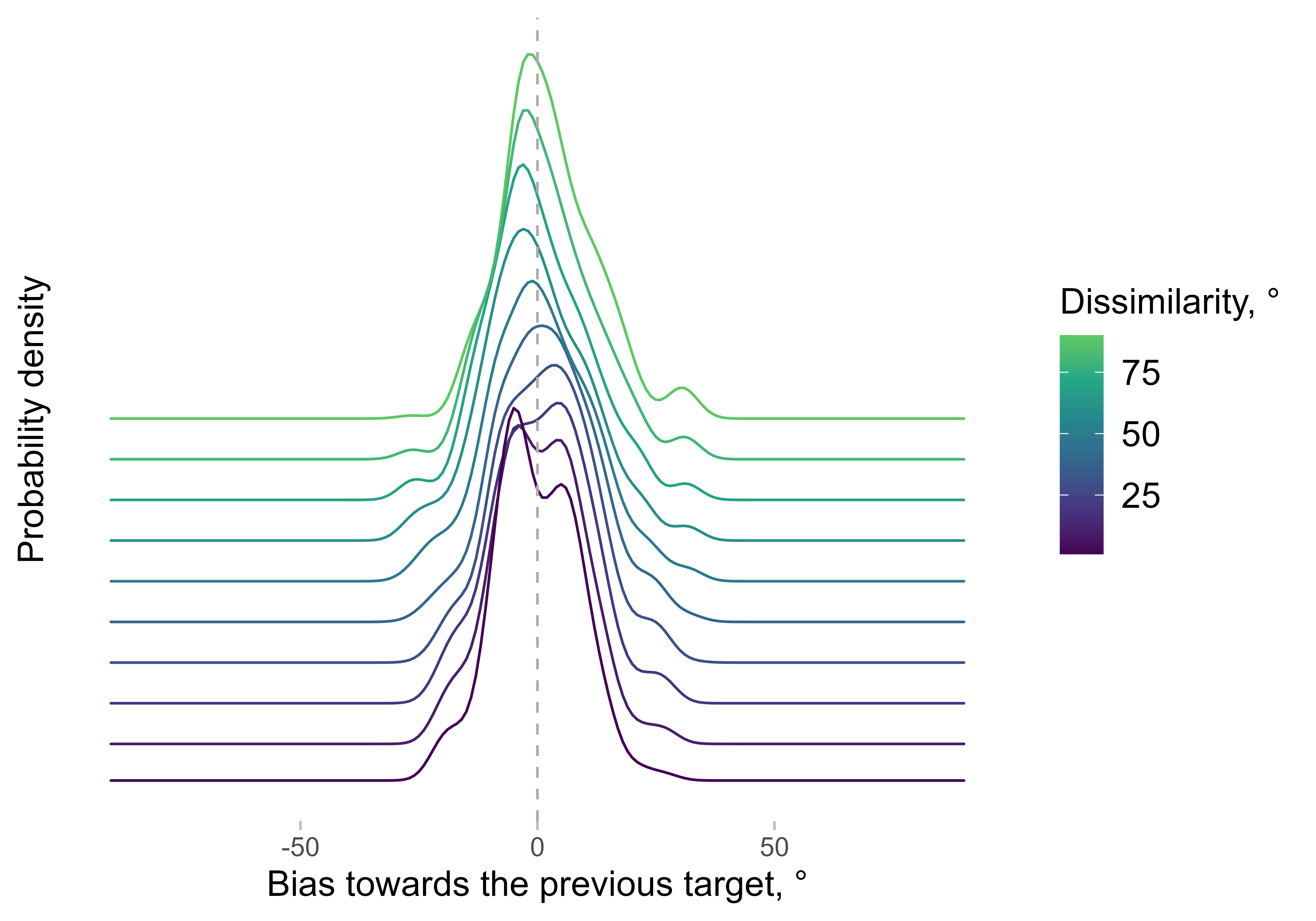

The x-axis shows the bias, which means that the errors are arranged in a way that positive bias corresponds to errors towards the previous target. For each dissimilarity step, the probabilities are estimated not only based on trials with exactly the same dissimilarity between the current and previous target, but also from all trials. The trials are weighted in a way that gives higher weight to trials with dissimilarities closer to the current value (technically, the function uses a Gaussian kernel with the standard deviation determined by weights_sd).

Note that the density is rarely a symmetric bell-shaped Gaussian, which makes using the mean as an overall estimator of bias problematic. This is based on observations from a single observer - other observers might have different patterns. This is one of the reasons why we started using asymmetry in the density, i.e. the difference between the left and right parts of the curve relative to zero.

We can then compute the asymmetry in the density (the main purpose of the function) by dropping the parameter return_full_density = T. We will also do it for all observers by specifying the parameter by:

err_dens <- density_asymmetry(data[!is.na(err_rel_to_prev_targ) & is_outlier == F],
  circ_space = 180, weights_sd = 10,
  xvar = "abs_diff_in_ori", yvar = "err_rel_to_prev_targ", by = c("observer")
)

We can then compute the statistics to test whether the bias is different from zero at different dissimilarity ranges (not shown here). Note that these ranges will depend on the smoothing window (or, more precisely, weights_sd - the standard deviations of a smoothing kernel). However, usually the exact range, in which the serial dependence is present, is not the main question of the study. The same issue will be present with other approaches (e.g., the bin width used when binning the data will have the same effect).

As a comparison, one can use binned errors:

data[, abs_diff_in_ori_bin := apastats::adv_cut(abs_diff_in_ori, cuts = seq(0, 90, 10), include_oob = T, num_labels = F, labels_at_means = T)]

mean_err <- apastats::get_superb_ci(data[!is.na(err_rel_to_prev_targ) & is_outlier == F], wid = "observer", within = "abs_diff_in_ori_bin", value_var = "err_rel_to_prev_targ")
#> Loading required namespace: superb
setDT(mean_err)
mean_err[, abs_diff_in_ori_bin := as.numeric(as.character(abs_diff_in_ori_bin))]

Putting them side by side:

p1 <- ggplot(err_dens[, mean_cl_normal(delta * 100), by = .(dist)], aes(x = dist, y = y, ymin = ymin, ymax = ymax)) +
  geom_line() +
  geom_ribbon(alpha = 0.1) +
  labs(y = "Asymmetry in error probability, %")

p2 <- ggplot(
  mean_err,
  aes(x = abs_diff_in_ori_bin, y = center, ymin = center + lowerwidth, ymax = center + upperwidth)
) +
  geom_line() +
  geom_pointrange() +
  labs(y = "Mean error, °")

(p1 + p2) &
  labs(x = "Absolute orientation difference, °") &
  geom_hline(yintercept = 0, linetype = 2) &
  scale_x_continuous(breaks = seq(0, 90, 30)) &
  coord_cartesian(xlim = c(0, 90))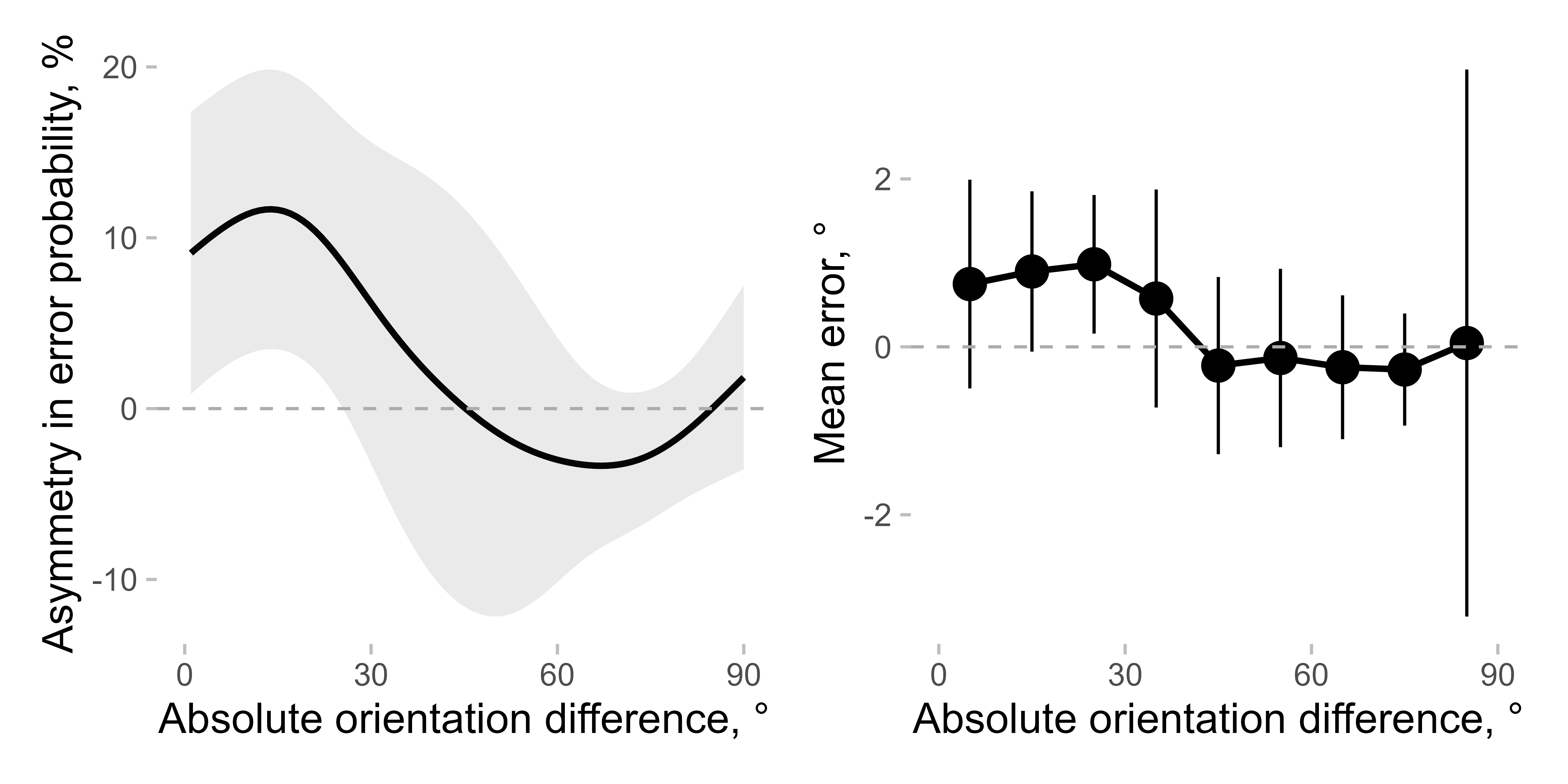

As you can see, the overall pattern is similar, although the effect seems clearer when using asymmetry in probability. Note also that the high confidence interval (CI) for the very last bin appears for the mean error but not for the asymmetry measure, as the latter is more robust than the former (Pascucci et al. dataset has fewer data points in this bin compared to the others).